

August 2021
Jo Tuffill introduces a new approach to calculating variances.
Variances is a tricky topic. Not only do students get confused with calculating them, they also find the interpretation aspect hard.
Students say, “I just can’t get those formulae in my head” or “I don’t understand the ‘should and did’ approach.”

Well, if you are one of those students for whom the tried and trusted approaches just don’t work, let me introduce you to an alternative.
Variances using diagrams
First of all, meet Carla and her candles.
Carla’s Candles are very on-trend for millennials, who want urban themed candles at an inexpensive price.
Until this year Carla has been selling through local shops and trade fairs, receiving trade price for her candles. But this year, due to Covid, she moved online. This has enabled her to sell direct to the public through her website linked to her Instagram and Facebook accounts.
Materials have been more difficult to get hold of and she has sometimes had to buy in smaller quantities than she would have liked. Carla has sourced alternative materials from different suppliers to alleviate the problem.
She normally has two staff members producing the candles for her once a week, but this year one member has had to shield and was not able to work.
Carla was able to furlough her under a government scheme. This has meant that her other staff member has been working two longer days.
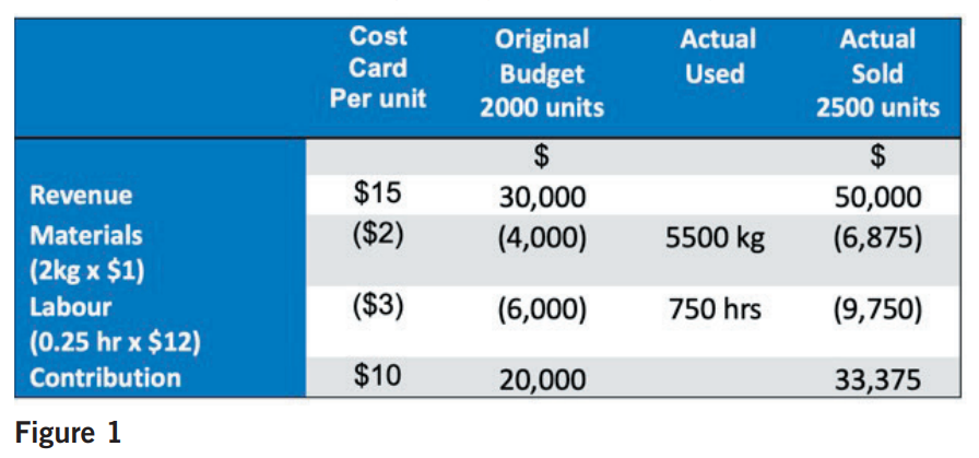
Figure 1 shows Carla’s results for 2020. Carla’s original budget is based on 2019 actual sales and costs operating over a 40-week year.
Flexing the budget to get meaningful comparisons for variance analysis
To be able to find the underlying performance of ‘Carla’s Candles’ we need to flex the original budget for the actual volume that was made and sold.
Comparing a budget of 2000 units to an actual of 2500 units will render any variances calculated, based on that budget, as meaningless.
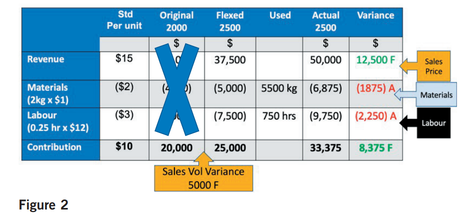
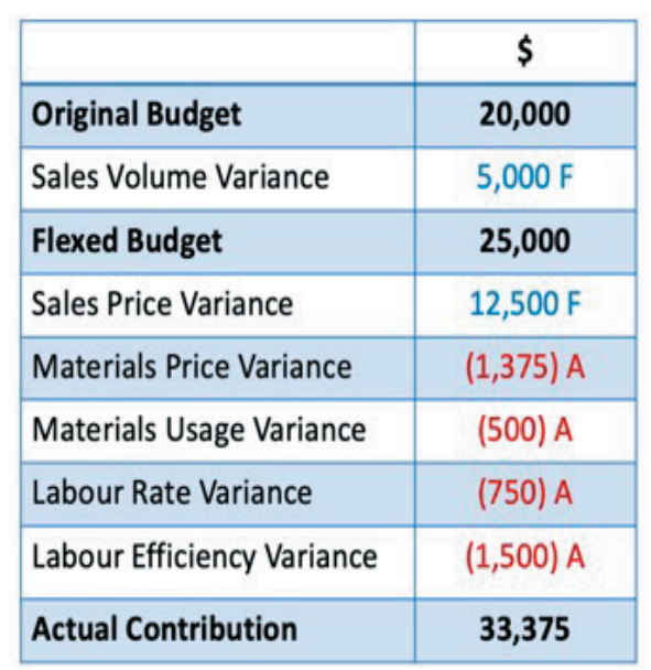
In figure 2, the flexed budget column is calculated by taking the standard per unit and multiplying it by the actual volume.
The sales volume variance is the difference between the original budget and the flexed budget (for actual volume) at the standard contribution.
This shows a $5,000 favourable variance and shows how much more contribution should be made at the higher volume of sales. We place a ‘cross’ over the original budget as that is now off limits!
All other variances are calculated from the flexed budget compared to actual results, being sales price, total materials and total labour variances.
Splitting the cost variances using triangles
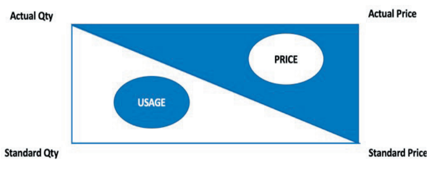
To understand the real story behind the cost variances we need to split and analyse the variances. Here in figure 3, the materials variance is split into price and usage using triangles. The total variance is represented by a rectangle and naming its top two corners with the actual quantity and price, then the bottom two corners with the standards you can visually see how the variance is split into two triangles and then calculated.
Figure 3 – Materials Variance part 1
In figure 4, we allocate the numbers to the corners using the standards and actuals given. You may need to calculate the price or usage quantity from the narrative but always be aware that you are flexing the standard usage quantity for the actual volume. The original budget is ‘off limits’.
Figure 4 – Materials Variance part 2
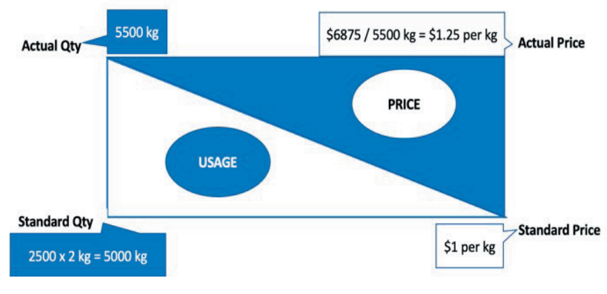
Using the triangles as your guide you take the difference between the vertical corners and multiply by the horizontal corner to get the variance.
• Price is the difference $1.25 to $1 ($0.25) multiplied by 5,500kg used resulting in $1,375 Adverse.
• Usage is the difference 5,500 kg to 5,000kg (500kg) multiplied by $1 price resulting in $500 Adverse.
• Total Variance is $1,375 A + $500 A = $1,875 Adverse.
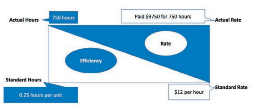
Have a go at applying this to the labour variance see figure 5. Calculate the variances for yourself using the diagram. See answers at the end of the article to check if you are correct.
Figure 5 – Labour Variance
What is the story of Carla’s Candles 2020 results?
Exam questions don’t just require you to calculate they also require you to interpret the variances. In order to gain the marks, you need to give relevance to your answers by using the scenario
Operating Statement
Sales Volume has increased due to online presence expanding her customer base outside the local market.
Sales Price to Carla has increased to $20 ($50,000/2500) from $15. She is no longer selling to trade at a 25% discount and is instead able to sell at full retail price direct to the end consumer.
Materials Price has increased by 25 cents per kg. Buying in lower quantities would mean higher delivery costs due to more deliveries in the year and perhaps missing out on quantity discounts. The alternative suppliers may also have charged a higher price as Carla is a new buyer. The actual market price of materials will also be increasing as supply has been restricted during the pandemic.
Materials Usage is adverse and could be due to an increase in wastage. The current standard is based on 2019 and maybe outdated. Carla has used alternative suppliers with perhaps a different grade of materials, and these may be more difficult to work with or of lower quality despite the price increase.
Labour Rate has increased on average by $1, this will be due to overtime hours. As the team has been halved the remaining staff member has been working a longer day over two days to fulfil the increase in demand. Carla will pay an increased rate for the overtime hours above the standard working day.
Labour Efficiency shows a significant adverse variance as two production staff work more efficiently than one. Tasks were probably split between them, matching skills to different parts of the production process. Now that only one member is available there will be a learning effect as they get up to speed and loss of efficiency from no longer having an assembly line. The materials usage and labour efficiency variance are linked here too.
New materials to work with will increase production time and taking on a new process will increase materials usage.
Conclusions
In this pandemic year Carla has seen significant change in her candles business. Being forced to move online has resulted in extending market reach and has cut out the intermediary allowing her to sell direct to the end customer at the full retail price. This has led to a significant increase in contribution of $17,500.
She has had her challenges, through the sourcing of supplies and a reduction in production efficiency. These have reduced her contribution by $4,125 (the total of the materials and labour variances). However, these issues are only temporary. Next year, she will have her trade customers back, supply chain issues will be resolved, and the staff member will return. Her challenge will now be to expand production to meet demand.
What do you think?
I hope the new approach works for you, where the usual techniques have failed. This concept can be applied to advanced variances too and for that lesson you need to join my online course.
• Jo Tuffill is the PM tutor with FME Learn Online. See www.jotuffill.co.uk
Answers to Figure 5
Rate is the difference ($9750/750 hours) $13 to $12 = $1 multiplied by 750 hours worked equals $750 A.
Efficiency is the difference 750 hours to (2500 units x 0.25 hour) 625 hours = 125 hours multiplied by $12 standard rate equals $1500 A.
